


- Bài 1: Giới thiệu Matplotlib
- Bài 2: Môi trường cài đặt
- Bài 3: Jupyter Notebook
- Bài 4: Pyplot API
- Bài 5: Khái niệm cơ bản về Plot
- Bài 6: PyLab
- Bài 7: Giao diện hướng đối tượng
- Bài 8: Figture và Axes
- Bài 9: Multiplots
- Bài 10: Hàm Subplots() và Subplot2grid()
- Bài 11: Grids
- Bài 12: Định dạng Axes
- Bài 13: Đặt giới hạn X và Y
- Bài 14: Trục đôi
- Bài 15: Bar Plot
- Bài 16: Histogram
- Bài 17: Pie Chart ( Biểu đồ tròn )
- Bài 18: Scatter Plot ( Biểu đồ phân tán )
- Bài 19: Contour Plot ( Đồ thị đường bao )
- Bài 20: Quiver Plot
- Bài 21: Box Plot ( Biểu đồ nén)
- Bài 22: Violin Plot
- Bài 23: Three-dimensional Plotting ( Biểu đồ 3 chiều )
- Bài 24: 3D Contour Plot ( Biểu đồ viền 3D )
- Bài 25: 3D Wireframe plot
- Bài 26: 3D Surface plot
- Bài 27: Làm việc với văn bản
- Bài 28: Biểu thức toán học
- Bài 29: Làm việc với ảnh
- Bài 30: Transforms ( Biến đổi trục )
Bài 28: Biểu thức toán học - Matplotib Cơ Bản
Đăng bởi: Admin | Lượt xem: 2944 | Chuyên mục: AI
1. Biểu thức toán học :
Sử dụng một tập con TeXmarkup trong bất kỳ chuỗi văn bản Matplotlib nào bằng cách đặt nó bên trong một cặp dấu đô la ($).
# math text
plt.title(r'$\alpha > \beta$')
Để tạo chỉ số dưới và chỉ số trên, hãy sử dụng các ký hiệu '_' và '^' -
r'$\alpha_i> \beta_i$'
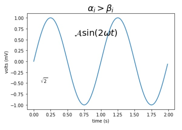
import numpy as np
import matplotlib.pyplot as plt
t = np.arange(0.0, 2.0, 0.01)
s = np.sin(2*np.pi*t)
plt.plot(t,s)
plt.title(r'$\alpha_i> \beta_i$', fontsize=20)
plt.text(0.6, 0.6, r'$\mathcal{A}\mathrm{sin}(2 \omega t)$', fontsize = 20)
plt.text(0.1, -0.5, r'$\sqrt{2}$', fontsize=10)
plt.xlabel('time (s)')
plt.ylabel('volts (mV)')
plt.show()Kết quả :
2. matplotlib.mathtext
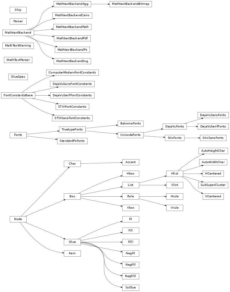
mathtext là một mô-đun để phân tích cú pháp một tập hợp con trong toán học TeX và vẽ chúng vào phần mềm phụ trợ matplotlib.
Để biết cách sử dụng nó, hãy xem Viết biểu thức toán học. Tài liệu này chủ yếu liên quan đến chi tiết triển khai.
Mô-đun sử dụng pyparsing để phân tích cú pháp biểu thức TeX.
Bản phân phối Bakoma của phông chữ TeX Computer Modern và phông chữ STIX được hỗ trợ. Có hỗ trợ thử nghiệm cho việc sử dụng các phông chữ tùy ý, nhưng kết quả có thể khác nhau nếu không có sự tinh chỉnh và chỉ số phù hợp cho các phông chữ đó.
3. Ví dụ :
import matplotlib.pyplot as plt
import subprocess
import sys
import re

# Selection of features following "Writing mathematical expressions" tutorial
mathtext_titles = {
    0: "Header demo",
    1: "Subscripts and superscripts",
    2: "Fractions, binomials and stacked numbers",
    3: "Radicals",
    4: "Fonts",
    5: "Accents",
    6: "Greek, Hebrew",
    7: "Delimiters, functions and Symbols"}
n_lines = len(mathtext_titles)

# Randomly picked examples
mathext_demos = {
    0: r"$W^{3\beta}_{\delta_1 \rho_1 \sigma_2} = "
    r"U^{3\beta}_{\delta_1 \rho_1} + \frac{1}{8 \pi 2} "
    r"\int^{\alpha_2}_{\alpha_2} d \alpha^\prime_2 \left[\frac{ "
    r"U^{2\beta}_{\delta_1 \rho_1} - \alpha^\prime_2U^{1\beta}_"
    r"{\rho_1 \sigma_2} }{U^{0\beta}_{\rho_1 \sigma_2}}\right]$",

    1: r"$\alpha_i > \beta_i,\ "
    r"\alpha_{i+1}^j = {\rm sin}(2\pi f_j t_i) e^{-5 t_i/\tau},\ "
    r"\ldots$",

    2: r"$\frac{3}{4},\ \binom{3}{4},\ \genfrac{}{}{0}{}{3}{4},\ "
    r"\left(\frac{5 - \frac{1}{x}}{4}\right),\ \ldots$",

    3: r"$\sqrt{2},\ \sqrt[3]{x},\ \ldots$",

    4: r"$\mathrm{Roman}\ , \ \mathit{Italic}\ , \ \mathtt{Typewriter} \ "
    r"\mathrm{or}\ \mathcal{CALLIGRAPHY}$",

    5: r"$\acute a,\ \bar a,\ \breve a,\ \dot a,\ \ddot a, \ \grave a, \ "
    r"\hat a,\ \tilde a,\ \vec a,\ \widehat{xyz},\ \widetilde{xyz},\ "
    r"\ldots$",

    6: r"$\alpha,\ \beta,\ \chi,\ \delta,\ \lambda,\ \mu,\ "
    r"\Delta,\ \Gamma,\ \Omega,\ \Phi,\ \Pi,\ \Upsilon,\ \nabla,\ "
    r"\aleph,\ \beth,\ \daleth,\ \gimel,\ \ldots$",

    7: r"$\coprod,\ \int,\ \oint,\ \prod,\ \sum,\ "
    r"\log,\ \sin,\ \approx,\ \oplus,\ \star,\ \varpropto,\ "
    r"\infty,\ \partial,\ \Re,\ \leftrightsquigarrow, \ \ldots$"}


def doall():
    # Colors used in mpl online documentation.
    mpl_blue_rvb = (191. / 255., 209. / 256., 212. / 255.)
    mpl_orange_rvb = (202. / 255., 121. / 256., 0. / 255.)
    mpl_grey_rvb = (51. / 255., 51. / 255., 51. / 255.)

    # Creating figure and axis.
    plt.figure(figsize=(6, 7))
    plt.axes([0.01, 0.01, 0.98, 0.90], facecolor="white", frameon=True)
    plt.gca().set_xlim(0., 1.)
    plt.gca().set_ylim(0., 1.)
    plt.gca().set_title("Matplotlib's math rendering engine",
                        color=mpl_grey_rvb, fontsize=14, weight='bold')
    plt.gca().set_xticklabels("", visible=False)
    plt.gca().set_yticklabels("", visible=False)

    # Gap between lines in axes coords
    line_axesfrac = (1. / (n_lines))

    # Plotting header demonstration formula
    full_demo = mathext_demos[0]
    plt.annotate(full_demo,
                 xy=(0.5, 1. - 0.59 * line_axesfrac),
                 color=mpl_orange_rvb, ha='center', fontsize=20)

    # Plotting features demonstration formulae
    for i_line in range(1, n_lines):
        baseline = 1 - (i_line) * line_axesfrac
        baseline_next = baseline - line_axesfrac
        title = mathtext_titles[i_line] + ":"
        fill_color = ['white', mpl_blue_rvb][i_line % 2]
        plt.fill_between([0., 1.], [baseline, baseline],
                         [baseline_next, baseline_next],
                         color=fill_color, alpha=0.5)
        plt.annotate(title,
                     xy=(0.07, baseline - 0.3 * line_axesfrac),
                     color=mpl_grey_rvb, weight='bold')
        demo = mathext_demos[i_line]
        plt.annotate(demo,
                     xy=(0.05, baseline - 0.75 * line_axesfrac),
                     color=mpl_grey_rvb, fontsize=16)

    for i in range(n_lines):
        s = mathext_demos[i]
        print(i, s)
    plt.show()


if '--latex' in sys.argv:
    # Run: python mathtext_examples.py --latex
    # Need amsmath and amssymb packages.
    fd = open("mathtext_examples.ltx", "w")
    fd.write("\\documentclass{article}\n")
    fd.write("\\usepackage{amsmath, amssymb}\n")
    fd.write("\\begin{document}\n")
    fd.write("\\begin{enumerate}\n")

    for i in range(n_lines):
        s = mathext_demos[i]
        s = re.sub(r"(?<!\\)\$", "$$", s)
        fd.write("\\item %s\n" % s)

    fd.write("\\end{enumerate}\n")
    fd.write("\\end{document}\n")
    fd.close()

    subprocess.call(["pdflatex", "mathtext_examples.ltx"])
else:
    doall()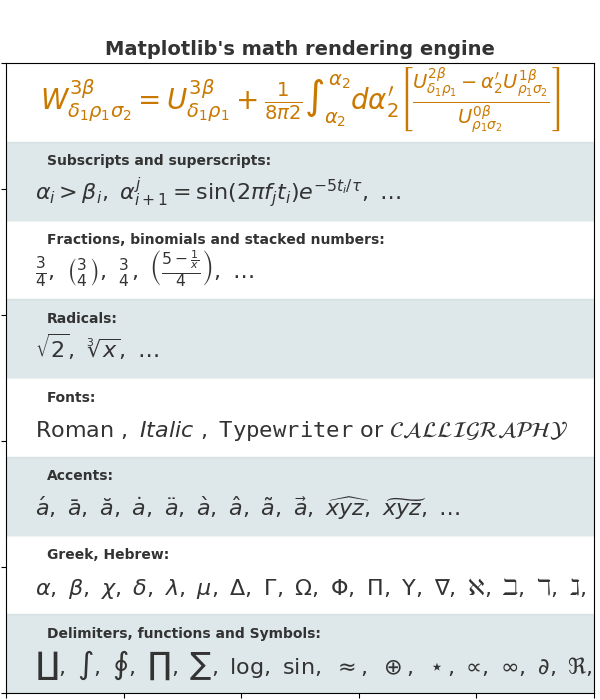
Kết quả :
0 $W^{3\beta}_{\delta_1 \rho_1 \sigma_2} = U^{3\beta}_{\delta_1 \rho_1} + \frac{1}{8 \pi 2} \int^{\alpha_2}_{\alpha_2} d \alpha^\prime_2 \left[\frac{ U^{2\beta}_{\delta_1 \rho_1} - \alpha^\prime_2U^{1\beta}_{\rho_1 \sigma_2} }{U^{0\beta}_{\rho_1 \sigma_2}}\right]$
1 $\alpha_i > \beta_i,\ \alpha_{i+1}^j = {\rm sin}(2\pi f_j t_i) e^{-5 t_i/\tau},\ \ldots$
2 $\frac{3}{4},\ \binom{3}{4},\ \genfrac{}{}{0}{}{3}{4},\ \left(\frac{5 - \frac{1}{x}}{4}\right),\ \ldots$
3 $\sqrt{2},\ \sqrt[3]{x},\ \ldots$
4 $\mathrm{Roman}\ , \ \mathit{Italic}\ , \ \mathtt{Typewriter} \ \mathrm{or}\ \mathcal{CALLIGRAPHY}$
5 $\acute a,\ \bar a,\ \breve a,\ \dot a,\ \ddot a, \ \grave a, \ \hat a,\ \tilde a,\ \vec a,\ \widehat{xyz},\ \widetilde{xyz},\ \ldots$
6 $\alpha,\ \beta,\ \chi,\ \delta,\ \lambda,\ \mu,\ \Delta,\ \Gamma,\ \Omega,\ \Phi,\ \Pi,\ \Upsilon,\ \nabla,\ \aleph,\ \beth,\ \daleth,\ \gimel,\ \ldots$
7 $\coprod,\ \int,\ \oint,\ \prod,\ \sum,\ \log,\ \sin,\ \approx,\ \oplus,\ \star,\ \varpropto,\ \infty,\ \partial,\ \Re,\ \leftrightsquigarrow, \ \ldots$Theo dõi VnCoder trên Facebook, để cập nhật những bài viết, tin tức và khoá học mới nhất!
- Bài 1: Giới thiệu Matplotlib
- Bài 2: Môi trường cài đặt
- Bài 3: Jupyter Notebook
- Bài 4: Pyplot API
- Bài 5: Khái niệm cơ bản về Plot
- Bài 6: PyLab
- Bài 7: Giao diện hướng đối tượng
- Bài 8: Figture và Axes
- Bài 9: Multiplots
- Bài 10: Hàm Subplots() và Subplot2grid()
- Bài 11: Grids
- Bài 12: Định dạng Axes
- Bài 13: Đặt giới hạn X và Y
- Bài 14: Trục đôi
- Bài 15: Bar Plot
- Bài 16: Histogram
- Bài 17: Pie Chart ( Biểu đồ tròn )
- Bài 18: Scatter Plot ( Biểu đồ phân tán )
- Bài 19: Contour Plot ( Đồ thị đường bao )
- Bài 20: Quiver Plot
- Bài 21: Box Plot ( Biểu đồ nén)
- Bài 22: Violin Plot
- Bài 23: Three-dimensional Plotting ( Biểu đồ 3 chiều )
- Bài 24: 3D Contour Plot ( Biểu đồ viền 3D )
- Bài 25: 3D Wireframe plot
- Bài 26: 3D Surface plot
- Bài 27: Làm việc với văn bản
- Bài 28: Biểu thức toán học
- Bài 29: Làm việc với ảnh
- Bài 30: Transforms ( Biến đổi trục )