


- Bài 1: Giới thiệu Matplotlib
- Bài 2: Môi trường cài đặt
- Bài 3: Jupyter Notebook
- Bài 4: Pyplot API
- Bài 5: Khái niệm cơ bản về Plot
- Bài 6: PyLab
- Bài 7: Giao diện hướng đối tượng
- Bài 8: Figture và Axes
- Bài 9: Multiplots
- Bài 10: Hàm Subplots() và Subplot2grid()
- Bài 11: Grids
- Bài 12: Định dạng Axes
- Bài 13: Đặt giới hạn X và Y
- Bài 14: Trục đôi
- Bài 15: Bar Plot
- Bài 16: Histogram
- Bài 17: Pie Chart ( Biểu đồ tròn )
- Bài 18: Scatter Plot ( Biểu đồ phân tán )
- Bài 19: Contour Plot ( Đồ thị đường bao )
- Bài 20: Quiver Plot
- Bài 21: Box Plot ( Biểu đồ nén)
- Bài 22: Violin Plot
- Bài 23: Three-dimensional Plotting ( Biểu đồ 3 chiều )
- Bài 24: 3D Contour Plot ( Biểu đồ viền 3D )
- Bài 25: 3D Wireframe plot
- Bài 26: 3D Surface plot
- Bài 27: Làm việc với văn bản
- Bài 28: Biểu thức toán học
- Bài 29: Làm việc với ảnh
- Bài 30: Transforms ( Biến đổi trục )
Bài 19: Contour Plot ( Đồ thị đường bao ) - Matplotib Cơ Bản
Đăng bởi: Admin | Lượt xem: 6724 | Chuyên mục: AI
1. Khái niệm cơ bản
Đồ thị đường bao (đôi khi được gọi là Đồ thị mức) là một cách để thể hiện một bề mặt ba chiều trên một mặt phẳng hai chiều. Nó vẽ biểu đồ hai biến dự báo X Y trên trục y và một biến phản ứng Z dưới dạng các đường bao. Những đường bao này đôi khi được gọi là z-slice hoặc giá trị iso-response.
Một đồ thị đường bao là thích hợp nếu bạn muốn xem đường viền Z thay đổi như thế nào dưới dạng hàm của hai đầu vào X và Y, sao cho Z = f (X, Y). Đường đồng mức hoặc đường cô lập của hàm hai biến là một đường cong mà hàm có giá trị không đổi.
Các biến độc lập x và y thường bị giới hạn trong một lưới thông thường gọi là meshgrid. Numpy.meshgrid tạo ra một lưới hình chữ nhật từ một mảng các giá trị x và một mảng các giá trị y.
API Matplotlib chứa hàm contour () và contourf () để vẽ đường đồng mức và đường bao đã tô tương ứng. Cả hai hàm đều cần ba tham số x, y và z.
import numpy as np
import matplotlib.pyplot as plt
xlist = np.linspace(-3.0, 3.0, 100)
ylist = np.linspace(-3.0, 3.0, 100)
X, Y = np.meshgrid(xlist, ylist)
Z = np.sqrt(X**2 + Y**2)
fig,ax=plt.subplots(1,1)
cp = ax.contourf(X, Y, Z)
fig.colorbar(cp) # Add a colorbar to a plot
ax.set_title('Filled Contours Plot')
#ax.set_xlabel('x (cm)')
ax.set_ylabel('y (cm)')
plt.show()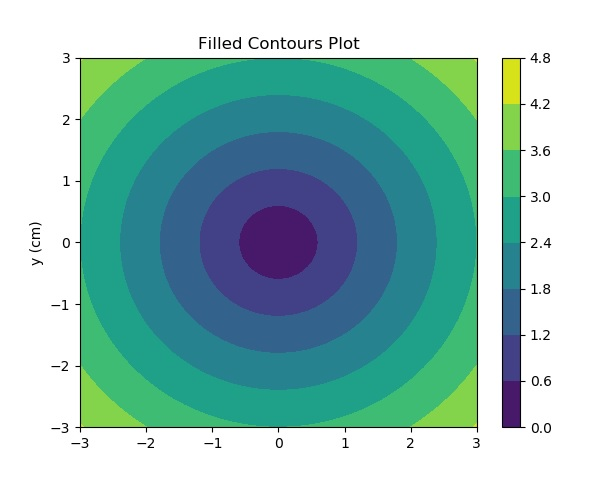
2. Ví dụ minh hoạ :
Ví dụ 1 :
Import các thư viện cần thiết :
import matplotlib
import numpy as np
import matplotlib.ticker as ticker
import matplotlib.pyplot as plt
Định nghĩa các giá trị :
delta = 0.025
x = np.arange(-3.0, 3.0, delta)
y = np.arange(-2.0, 2.0, delta)
X, Y = np.meshgrid(x, y)
Z1 = np.exp(-X**2 - Y**2)
Z2 = np.exp(-(X - 1)**2 - (Y - 1)**2)
Z = (Z1 - Z2) * 2
Tạo nhãn đường viền bằng cách sử dụng các class float như sau :
# Define a class that forces representation of float to look a certain way
# This remove trailing zero so '1.0' becomes '1'


class nf(float):
    def __repr__(self):
        s = f'{self:.1f}'
        return f'{self:.0f}' if s[-1] == '0' else s


# Basic contour plot
fig, ax = plt.subplots()
CS = ax.contour(X, Y, Z)

# Recast levels to new class
CS.levels = [nf(val) for val in CS.levels]

# Label levels with specially formatted floats
if plt.rcParams["text.usetex"]:
    fmt = r'%r \%%'
else:
    fmt = '%r %%'

ax.clabel(CS, CS.levels, inline=True, fmt=fmt, fontsize=10)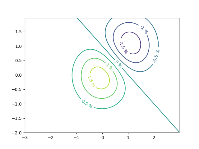
Kết quả :
<a list of 7 text.Text objects>Gắn nhãn các đường viền bằng các chuỗi tùy ý bằng cách sử dụng dictionary
fig1, ax1 = plt.subplots()

# Basic contour plot
CS1 = ax1.contour(X, Y, Z)

fmt = {}
strs = ['first', 'second', 'third', 'fourth', 'fifth', 'sixth', 'seventh']
for l, s in zip(CS1.levels, strs):
    fmt[l] = s

# Label every other level using strings
ax1.clabel(CS1, CS1.levels[::2], inline=True, fmt=fmt, fontsize=10)
Kết quả :
<a list of 3 text.Text objects>Sử dụng Formatter :
fig2, ax2 = plt.subplots()

CS2 = ax2.contour(X, Y, 100**Z, locator=plt.LogLocator())
fmt = ticker.LogFormatterMathtext()
fmt.create_dummy_axis()
ax2.clabel(CS2, CS2.levels, fmt=fmt)
ax2.set_title("$100^Z$")

plt.show()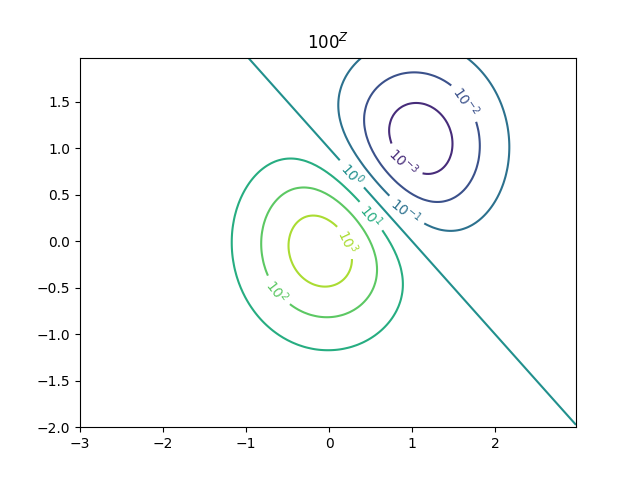
Ví dụ 2 : Cách sử dụng phương thức axis.Axes.contourf () để tạo các đồ thị đường bao đã điền.
import numpy as np
import matplotlib.pyplot as plt
origin = 'lower'
delta = 0.025
x = y = np.arange(-3.0, 3.01, delta)
X, Y = np.meshgrid(x, y)
Z1 = np.exp(-X**2 - Y**2)
Z2 = np.exp(-(X - 1)**2 - (Y - 1)**2)
Z = (Z1 - Z2) * 2
nr, nc = Z.shape
# put NaNs in one corner:
Z[-nr // 6:, -nc // 6:] = np.nan
# contourf will convert these to masked
Z = np.ma.array(Z)
Z[:nr // 6, :nc // 6] = np.ma.masked
# mask a circle in the middle:
interior = np.sqrt(X**2 + Y**2) < 0.5
Z[interior] = np.ma.masked
# We are using automatic selection of contour levels;
# this is usually not such a good idea, because they don't
# occur on nice boundaries, but we do it here for purposes
# of illustration.
fig1, ax2 = plt.subplots(constrained_layout=True)
CS = ax2.contourf(X, Y, Z, 10, cmap=plt.cm.bone, origin=origin)
# Note that in the following, we explicitly pass in a subset of
# the contour levels used for the filled contours. Alternatively,
# We could pass in additional levels to provide extra resolution,
# or leave out the levels kwarg to use all of the original levels.
CS2 = ax2.contour(CS, levels=CS.levels[::2], colors='r', origin=origin)
ax2.set_title('Nonsense (3 masked regions)')
ax2.set_xlabel('word length anomaly')
ax2.set_ylabel('sentence length anomaly')
# Make a colorbar for the ContourSet returned by the contourf call.
cbar = fig1.colorbar(CS)
cbar.ax.set_ylabel('verbosity coefficient')
# Add the contour line levels to the colorbar
cbar.add_lines(CS2)
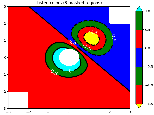
fig2, ax2 = plt.subplots(constrained_layout=True)
# Now make a contour plot with the levels specified,
# and with the colormap generated automatically from a list
# of colors.
levels = [-1.5, -1, -0.5, 0, 0.5, 1]
CS3 = ax2.contourf(X, Y, Z, levels,
colors=('r', 'g', 'b'),
origin=origin,
extend='both')
# Our data range extends outside the range of levels; make
# data below the lowest contour level yellow, and above the
# highest level cyan:
CS3.cmap.set_under('yellow')
CS3.cmap.set_over('cyan')
CS4 = ax2.contour(X, Y, Z, levels,
colors=('k',),
linewidths=(3,),
origin=origin)
ax2.set_title('Listed colors (3 masked regions)')
ax2.clabel(CS4, fmt='%2.1f', colors='w', fontsize=14)
# Notice that the colorbar command gets all the information it
# needs from the ContourSet object, CS3.
fig2.colorbar(CS3)
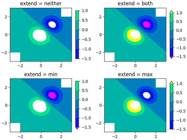
# Illustrate all 4 possible "extend" settings:
extends = ["neither", "both", "min", "max"]
cmap = plt.cm.get_cmap("winter")
cmap.set_under("magenta")
cmap.set_over("yellow")
# Note: contouring simply excludes masked or nan regions, so
# instead of using the "bad" colormap value for them, it draws
# nothing at all in them. Therefore the following would have
# no effect:
# cmap.set_bad("red")
fig, axs = plt.subplots(2, 2, constrained_layout=True)
for ax, extend in zip(axs.ravel(), extends):
cs = ax.contourf(X, Y, Z, levels, cmap=cmap, extend=extend, origin=origin)
fig.colorbar(cs, ax=ax, shrink=0.9)
ax.set_title("extend = %s" % extend)
ax.locator_params(nbins=4)
plt.show()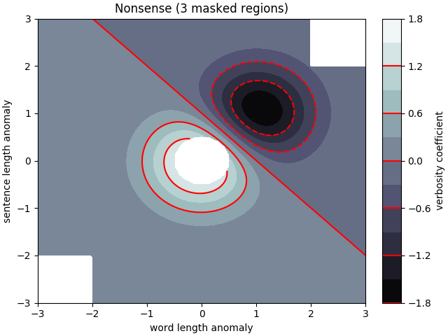
Theo dõi VnCoder trên Facebook, để cập nhật những bài viết, tin tức và khoá học mới nhất!
- Bài 1: Giới thiệu Matplotlib
- Bài 2: Môi trường cài đặt
- Bài 3: Jupyter Notebook
- Bài 4: Pyplot API
- Bài 5: Khái niệm cơ bản về Plot
- Bài 6: PyLab
- Bài 7: Giao diện hướng đối tượng
- Bài 8: Figture và Axes
- Bài 9: Multiplots
- Bài 10: Hàm Subplots() và Subplot2grid()
- Bài 11: Grids
- Bài 12: Định dạng Axes
- Bài 13: Đặt giới hạn X và Y
- Bài 14: Trục đôi
- Bài 15: Bar Plot
- Bài 16: Histogram
- Bài 17: Pie Chart ( Biểu đồ tròn )
- Bài 18: Scatter Plot ( Biểu đồ phân tán )
- Bài 19: Contour Plot ( Đồ thị đường bao )
- Bài 20: Quiver Plot
- Bài 21: Box Plot ( Biểu đồ nén)
- Bài 22: Violin Plot
- Bài 23: Three-dimensional Plotting ( Biểu đồ 3 chiều )
- Bài 24: 3D Contour Plot ( Biểu đồ viền 3D )
- Bài 25: 3D Wireframe plot
- Bài 26: 3D Surface plot
- Bài 27: Làm việc với văn bản
- Bài 28: Biểu thức toán học
- Bài 29: Làm việc với ảnh
- Bài 30: Transforms ( Biến đổi trục )