Bài 13: Đặt giới hạn X và Y

Bài 13: Đặt giới hạn X và Y - Matplotib Cơ Bản

Đăng bởi: Admin | Lượt xem: 2328 | Chuyên mục: AI

1. Khái niệm :

Matplotlib tự động đi từ các giá trị tối thiểu và lớn nhất của các biến được hiển thị dọc theo trục x, y (và trục z trong trường hợp biểu đồ 3D) của một biểu đồ. Tuy nhiên, có thể đặt giới hạn một cách rõ ràng bằng cách sử dụng hàm set_xlim () và set_ylim ().

Trong biểu đồ sau, các giới hạn được tự động chia tỷ lệ của trục x và y được hiển thị:

import matplotlib.pyplot as plt
fig = plt.figure()
a1 = fig.add_axes([0,0,1,1])
import numpy as np
x = np.arange(1,10)
a1.plot(x, np.exp(x))
a1.set_title('exp')
plt.show()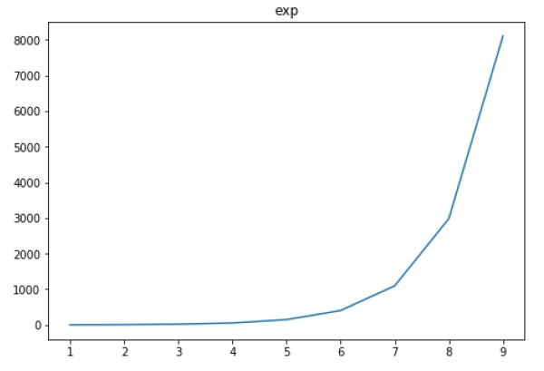

Bây giờ chỉnh giới hạn trên trục x thành (0 đến 10) và trục y (0 đến 10000) -

import matplotlib.pyplot as plt
fig = plt.figure()
a1 = fig.add_axes([0,0,1,1])
import numpy as np
x = np.arange(1,10)
a1.plot(x, np.exp(x),'r')
a1.set_title('exp')
a1.set_ylim(0,10000)
a1.set_xlim(0,10)
plt.show()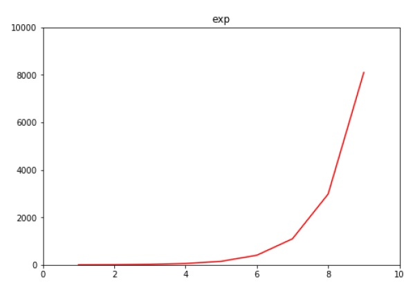

2. Ví dụ :

Ví dụ 1 : Broken Barh

import matplotlib.pyplot as plt

fig, ax = plt.subplots()
ax.broken_barh([(110, 30), (150, 10)], (10, 9), facecolors='tab:blue')
ax.broken_barh([(10, 50), (100, 20), (130, 10)], (20, 9),
               facecolors=('tab:orange', 'tab:green', 'tab:red'))
ax.set_ylim(5, 35)
ax.set_xlim(0, 200)
ax.set_xlabel('seconds since start')
ax.set_yticks([15, 25])
ax.set_yticklabels(['Bill', 'Jim'])
ax.grid(True)
ax.annotate('race interrupted', (61, 25),
            xytext=(0.8, 0.9), textcoords='axes fraction',
            arrowprops=dict(facecolor='black', shrink=0.05),
            fontsize=16,
            horizontalalignment='right', verticalalignment='top')

plt.show()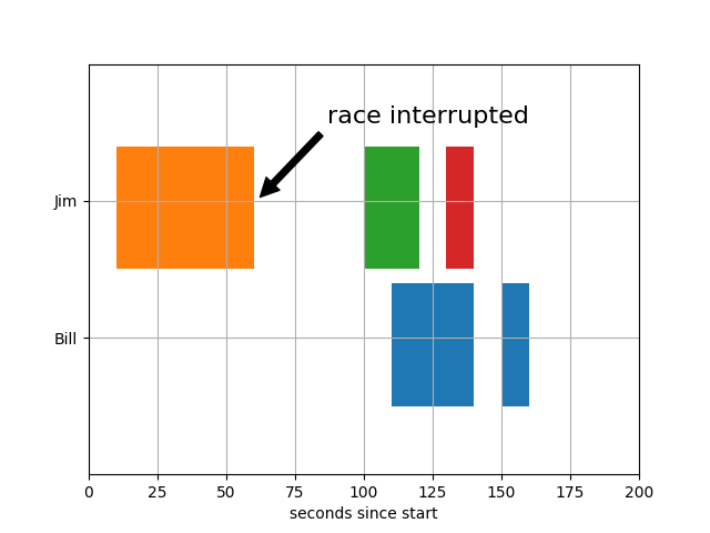

Ví dụ 2 : CSD Demo

import numpy as np
import matplotlib.pyplot as plt


fig, (ax1, ax2) = plt.subplots(2, 1)
# make a little extra space between the subplots
fig.subplots_adjust(hspace=0.5)

dt = 0.01
t = np.arange(0, 30, dt)

# Fixing random state for reproducibility
np.random.seed(19680801)


nse1 = np.random.randn(len(t))                 # white noise 1
nse2 = np.random.randn(len(t))                 # white noise 2
r = np.exp(-t / 0.05)

cnse1 = np.convolve(nse1, r, mode='same') * dt   # colored noise 1
cnse2 = np.convolve(nse2, r, mode='same') * dt   # colored noise 2

# two signals with a coherent part and a random part
s1 = 0.01 * np.sin(2 * np.pi * 10 * t) + cnse1
s2 = 0.01 * np.sin(2 * np.pi * 10 * t) + cnse2

ax1.plot(t, s1, t, s2)
ax1.set_xlim(0, 5)
ax1.set_xlabel('time')
ax1.set_ylabel('s1 and s2')
ax1.grid(True)

cxy, f = ax2.csd(s1, s2, 256, 1. / dt)
ax2.set_ylabel('CSD (db)')
plt.show()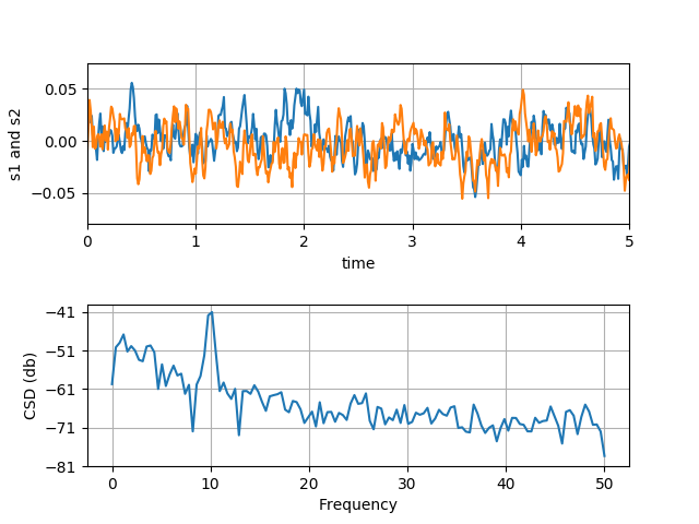

Ví dụ 3 : EventCollection Demo

import matplotlib.pyplot as plt
from matplotlib.collections import EventCollection
import numpy as np

# Fixing random state for reproducibility
np.random.seed(19680801)

# create random data
xdata = np.random.random([2, 10])

# split the data into two parts
xdata1 = xdata[0, :]
xdata2 = xdata[1, :]

# sort the data so it makes clean curves
xdata1.sort()
xdata2.sort()

# create some y data points
ydata1 = xdata1 ** 2
ydata2 = 1 - xdata2 ** 3

# plot the data
fig = plt.figure()
ax = fig.add_subplot(1, 1, 1)
ax.plot(xdata1, ydata1, color='tab:blue')
ax.plot(xdata2, ydata2, color='tab:orange')

# create the events marking the x data points
xevents1 = EventCollection(xdata1, color='tab:blue', linelength=0.05)
xevents2 = EventCollection(xdata2, color='tab:orange', linelength=0.05)

# create the events marking the y data points
yevents1 = EventCollection(ydata1, color='tab:blue', linelength=0.05,
                           orientation='vertical')
yevents2 = EventCollection(ydata2, color='tab:orange', linelength=0.05,
                           orientation='vertical')

# add the events to the axis
ax.add_collection(xevents1)
ax.add_collection(xevents2)
ax.add_collection(yevents1)
ax.add_collection(yevents2)

# set the limits
ax.set_xlim([0, 1])
ax.set_ylim([0, 1])

ax.set_title('line plot with data points')

# display the plot
plt.show()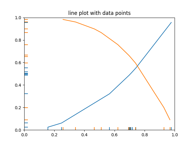

Ví dụ 4 : Join Styles và Cap Styles

Ví dụ này minh họa các kiểu nối và kiểu mũ có sẵn.

Cả hai đều được sử dụng trong Line2D và các Bộ sưu tập khác nhau từ matplotlib.collections cũng như một số hàm tạo ra các bộ sưu tập này, ví dụ: âm mưu.

a. Join Styles :

import numpy as np
import matplotlib.pyplot as plt


def plot_angle(ax, x, y, angle, style):
    phi = np.radians(angle)
    xx = [x + .5, x, x + .5*np.cos(phi)]
    yy = [y, y, y + .5*np.sin(phi)]
    ax.plot(xx, yy, lw=12, color='tab:blue', solid_joinstyle=style)
    ax.plot(xx, yy, lw=1, color='black')
    ax.plot(xx[1], yy[1], 'o', color='tab:red', markersize=3)


fig, ax = plt.subplots(figsize=(8, 6))
ax.set_title('Join style')

for x, style in enumerate(['miter', 'round', 'bevel']):
    ax.text(x, 5, style)
    for y, angle in enumerate([20, 45, 60, 90, 120]):
        plot_angle(ax, x, y, angle, style)
        if x == 0:
            ax.text(-1.3, y, f'{angle} degrees')
ax.text(1, 4.7, '(default)')

ax.set_xlim(-1.5, 2.75)
ax.set_ylim(-.5, 5.5)
ax.xaxis.set_visible(False)
ax.yaxis.set_visible(False)
plt.show()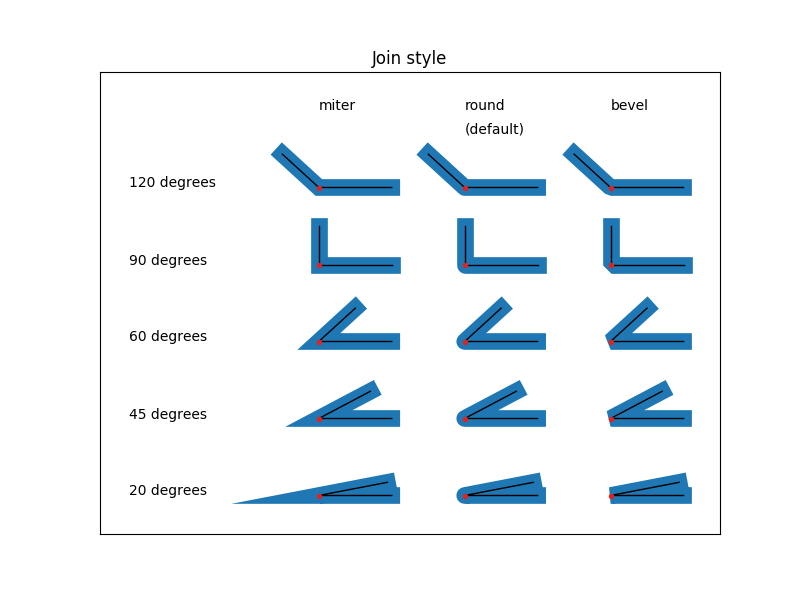

b. Cap styles :

fig, ax = plt.subplots(figsize=(8, 2))
ax.set_title('Cap style')

for x, style in enumerate(['butt', 'round', 'projecting']):
    ax.text(x, 1, style)
    xx = [x, x+0.5]
    yy = [0, 0]
    ax.plot(xx, yy, lw=12, color='tab:blue', solid_capstyle=style)
    ax.plot(xx, yy, lw=1, color='black')
    ax.plot(xx, yy, 'o', color='tab:red', markersize=3)
ax.text(2, 0.7, '(default)')

ax.set_ylim(-.5, 1.5)
ax.xaxis.set_visible(False)
ax.yaxis.set_visible(False)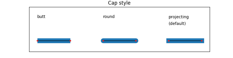

Bài tiếp theo: Trục đôi >>

Theo dõi VnCoder trên Facebook, để cập nhật những bài viết, tin tức và khoá học mới nhất!